In the previous chapter we discovered a way of avoiding the lack of flexibility of Bézier curves through the use of rational curves. Even so, the flexibility that the weights of the rational curves provide us is much limited. Instead of covering the whole curve with just one parametrization (polynomial or rational), we could use several of them. Then we achieve more flexibility: when we modify a parametrization, we just modify the corresponding part of the graphic.
First we shall study how to build C1 piecewise parabolas and C2 and C1 piecewise cubics as a prior step to a more general procedure.
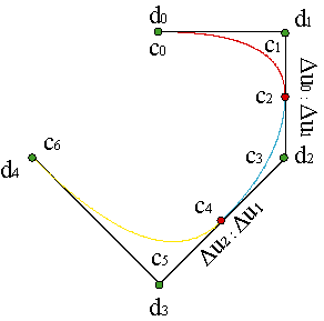
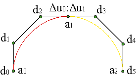
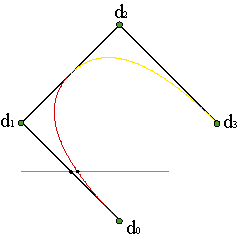
Consider a plane curve formed by N parabolic pieces. We have a collection of vertices {c0,..., c2N}, such that {c0,c1,c2} is the control polygon of the first piece, {c2,c3,c4} is the polygon of the second one, {c2(i-1),c2i-1,c2i}, the one for the i-th, and {c2N-2,c2N-1,c2N}, the last one.
Each polygon defines a parametrization over an interval. The first piece is defined over the interval [u0,u1], the second one over [u1,u2], the i-th over [ui-1,ui] and the last one over [uN-1,uN].
If we want the piecewise curve to be C1 all over the interval [u0,uN], we must demand it for each value u = ui, as seen in the second chapter:
| (1) |
That is: that vectors c2i-1c2i y c2ic2i+1 are parallel and in proportion Δui-1:Δui.
The expressions (1) collapse if we allow the user to modify (move) all the vertices. Therefore, if we want the class of differentiability unchanged, all we have to do is to allow the modification (movement) of those vertices which will not affect that condition.
Having this in mind, we can view the definition (1) as the definition of the vertex c2i, given the vertices c2i-1, c2i+1,
| (2) |
These expressions bring back the fact that the simple ratio of the points c2i-1, c2i, c2i+1 is [c2i-1,c2i,c2i+1] = Δui-1/Δui.
Summing up, the only data that must be given to the user in order to modify freely the curve without changing the smoothness condition are:
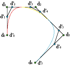
Hence: N+2 vertices, corresponding to the fact that we have 2N+1 vertices and N-1 differentiability conditions at the unions. Example
We refer to those vertices as {d0,...,dN+1},
| (3) |
This set of vertices is the so-called B-spline control polygon of the piecewise polynomial curve.
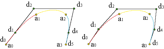
The construction of the C1 class piecewise parabola can be used for interpolating a C1 class curve that passes through N+1 points of the plane, a0,...,aN, for some given values of the parameter u, ai = c(ui). We just have to solve a linear system of equations c2i = ai,
| |||||||||||||||||||||||
This is underdetermined: we have N-1 linear equations for N unknowns, the vertices d1,...,dN.
We need another condition besides the values xi: = (Δui-1+Δui) ai.
We need to fix, for instance, a tangent in one of the pieces.
If the curve is closed, c0 = c2N+2, each and every even vertex can be found from the odd adjacent ones due to the relation (2). Hence, it is only necessary to give these ones, {c1,...,c2i-1,...,c2N+1}.
The initial-final vertex can be found as a particular case:
| ||||||||||||||||||||||
The B-spline polygon, {d0,...,dN}, is formed by the interior vertices , d0 = c2N+1, di = c2i-1, i = 1,...,N.
The matrix for this problem is regular for even N. As a consequence, this method enables us to find a unique solution for the interpolation problem for an odd number of points. Hence, it does not seem to be a reliable method. Example
Notice that, as the parabola is a plane conic section, this construction is valid only for plane curves.
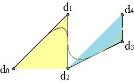
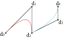
In order to solve the problem in the space, we have to use cubic curves. We try to build a C2 class curve of N pieces. The vertices of our control polygons will be {c0,...,c3N}, of which {c3(i-1),c3i-2,c3i-1,c3i} correspond to the i-th piece, defined over the interval [ui-1,ui].
We impose the parametrization to be C2 class in u = ui, union of the pieces i-th and (i+1)-th. As in the previous item, this is the C1 condition
| (6) |
| (7) |
that is to say: the vectors c3i-1c3i y c3ic3i+1 are parallel and in proportion Δui-1:Δui.
Finally, the condition of continuity of the second derivatives (see chapter 2) applied to the knot ui give us as information that the vectors c3i-2c3i-1 and c3i-1di are in ratio Δui-1:Δui, the same as the vectors di c3i+1 and c3i+1 c3i+2.
Applying this condition to the knot ui+1 we get another relation. The vectors c3i+1c3i+2 and c3i+2di+1 are in ratio Δui:Δui+1.
And from the knot ui-1 we learn di-1 c3i-2 and c3i-2c3i-1 are in ratio Δui-2:Δui-1.
Using all this information, we can express the vertices c3i-1, c3i+1 in terms of the new points we have introduced,
| ||||||||||||||||||||||
Combining this result with (7) allows us to find all the vertices of the piecewise curve having as a starting point the points d1,...,dN-1, ensuring that the parametrization is C2.
We left behind the vertices that are not adjacent to any union, i.e., the initial vertices, c0, c1, and the final ones, c3N-1, c3N, that cannot be found through any of these relations.
We denote d-1: = c0, d0: = c1, dN: = c3N-1, dN+1: = c3N, in order to complete the list of vertices. The remaining vertices, c2, c3N-2 can be found from (8) taking Δu-1 and ΔuN equal to zero.
Actually, the usual notation is the correlative one from 0 to N+2. In that case we have to move all the indexes in one unity. We follow this notation from now on.
In the case of closed curves, there is no need to add more points, and all the vertices can be found from (7) y (8).
Consequently, we can encode the piecewise curve in the B-spline control polygon, {d0,...,dN+2} and the sequence of knots {u0,...,uN}. Thus, the user will be able to modify the curve without changing its properties of differentiability.
Replacing the expressions of the vertices c3i-1 and c3i+1 in (7),
| ||||||||||
| ||||||||||
| ||||||||||||
| |||||||||||
Notice that c3i depends on three consecutive vertices of the B-spline polygon.
This relation is helpful for solving the interpolation problem: given N+1 points a0,..., aN and knots {u0,...,uN}, find the C2 piecewise cubic such that c(ui) = ai.
The problem can be reduced to the linear system (9), where the data are:
We have, then, N+3 unknowns for N+1 data, so the system has two free parameters (two degrees of freedom), for instance, d1 y dN+1.
It can be proven that the system has rank N+1, and hence the problem has a unique solution (but we have to fix those vertices first).
There are many ways of fixing vertices by imposing conditions on the curve.
One of them, imposing the so-called natural conditions, that mimic the physical behaviour of a real spline, which tends to a straight line near the endings. Therefore:
| (10) |
Notwithstanding, these conditions are not much appreciated in design, because they cause that the curve is too straight at the endpoints.
Another option is choosing the tangent directions at the endpoints, c'(u0), c'(uN). These will determine the vertices d1, dN+1,
| ||||||||
if we take into account that d0 = a0, dN+2 = aN,
| |||||||||
This will reduce the linear system to N-1 equations for N-1 unknowns.
An alternative way of choosing the tangent directions is given by Bessel conditions: choosing c'(u0) as the value of the derivative in the origin of the parabola that passes through the points a0, a1, a2 and, analogously, c'(uN) will be the derivative at uN of the parabola that interpolates aN-2, aN-1, aN.
The Bessel tangents provide us much better results than natural conditions. Example
In the case of closed curves, no additional data are needed. The system is closed naturally in a periodic way.
Summing up: in order to build curves of degree n of N pieces of Cn-1 class, the Bézier curves give us nN+1 vertices from their control polygons, but we have n-1 conditions of differentiability at the N-1 unions. Hence, we have nN+1-(N-1)(n-1) = N+n degrees of freedom.
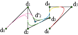
An alternative problem for piecewise cubic interpolation could be:
Assume that we have N+1 points {a0,...,aN} and N+1 vectors {v0,...,vN} and we want to trace the interpolating curve c(u) such that c(ui) = ai, c'(ui) = vi, i = 0,...,N, for an increasing sequence of values of the parameter u, {u0,...,uN}.
A simple solution for this problem could be a C1 piecewise cubic with N pieces. As in the previous example, the curve requires 3N+1 vertices {c0,...,c3N}, of which N+1, the endpoints of the cubics, are determined by the conditions c3i = ai, i = 0,..., N. The rest of them are determined by the tangent directions.
Having in mind the previous expressions:
| |||||||||||||||||
respectively for the initial and final points of each piece. From here, we get the interior vertices of each polygon,
| ||||||||||||||||||
Hence, in this case there are no additional degrees of freedom and the curve is clearly determined.
However, in order to encode the information of the curves, it is not necessary to give all the vertices of the curve but only the inner ones, due to the fact that the outer ones can be found from the previous relations, but the initial and final vertices, c0, c3N.
Therefore, the curve can be characterized by a sequence of knots {u0,..., uN} and vertices of the B-spline polygon, {d0,..., d2N+1}, given by d0: = c0, d2i-1 = c3i-2, d2i = c3i-1, i = 1,..., N, d2N+1 = c3N,
| |||||||
In case we are interpolating with closed curves it is even easier: the expressions (12-13) are still valid even for the cases i = 0,N for Δu-1: = ΔuN, but we need in addition one more knot, uN+1, the one who closes the curve with the conditions a0 = c(uN+1), v0 = c'(uN+1).
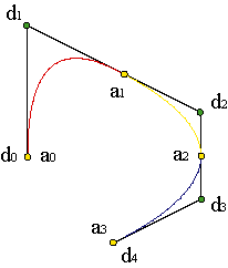
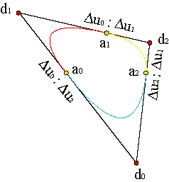
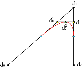
Consider a parabola parametrized on an interval [u1,u2] by c(u). Considering that blossoms are multiaffine, we can express c(u) as another step of the de Casteljau algorithm,
| ||||||||
and with another step of the de Casteljau algorithm, but this time using auxiliary knots u0,u3,
| ||||||||||||||||||||||||||
Consequently, we have expressed every point of c(u) as function of three vertices, c[u0,u1], c[u1,u2], c[u2,u3], which, in general, the curve is not passing through. Example
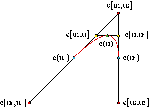
Notice that, for u0 = u1, u3 = u2, we recover the de Casteljau algorithm for the control polygon {c0 = c[u1,u1], c1 = c[u1,u2], c2 = c[u2,u2]}.
Therefore, we have just generalized the de Casteljau algorithm by introducing two auxiliary knots.
In order to make all the terms positive in the parametrization, we define it over the interval [u1,u2]. We have done this for linking different pieces of polynomial curves.
Summing up, the steps of the algorithm are:
| ||||||||||||||||||||
The B-spline polygon for the parabola is formed by the vertices:
{d0: = c[u0,u1],d1: = c[u1,u2],d2: = c[u2,u3]}.
This is the de Boor algorithm for a parabolic curve with just one piece. The algorithm can be generalized to curves of degree n having just one piece. The polygon will be formed by n+1 vertices, corresponding to a polynomial curve of degree n, {d0,...,dn}, for di = c[ui,...,ui+n-1].
The sequence of knots will be formed by 2n parameter values {u0,...,u2n-1}. Example
Finally, the de Boor algorithm consists on using in a iterated way the de Casteljau algorithm,
| |||||||||||||||||||||||||||||||||||||||||
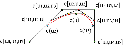
For: c(u) = dn)0(u). The parametrization is defined over the interval [un-1,un]. Example
The blossom for the de Boor algorithm can be formed easily. For the polygon of a curve of degree n, {d0,...,dn}, and a sequence of knots, {u0,...,u2n-1}, the blossom can be evaluated at the parameter values v1,...,vn ,
| ||||||||
| ||||||||||||
| ||||||||
| ||||||||||
| ||||||||||
| ||||||||
| ||||||||||
| |||||||||||
The blossom is still symmetric, despite its apparent asymmetry.
The blossom again returns the correct values of the vertices of the control polygon,
| ||||
By introducing the de Boor algorithm for polynomial curves of just one piece, we have just changed the set of points which we calculated the blossom with. Instead of using {c0,...,cn} for the de Casteljau algorithm, we use {d0,...,dn} for the de Boor one. But the blossom is still the same.
The blossom gives us a simple mechanism for passing from one scheme to the other.
For instance, if we have a B-spline polygon of a curve of degree n, {d0,...,dn}, the control polygon as a Bézier curve will be
| ||||
This could seem superfluous but we shall see the importance for curves of several pieces in the next section.
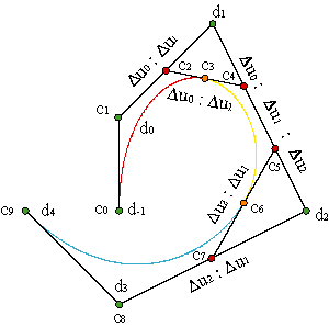
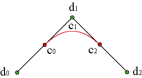
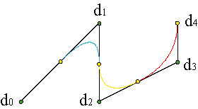
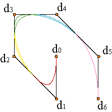
The de Boor algorithm can be easily used for curves consisting on N parabolic pieces of degree n. Consider a set of vertices {d0,...,dn+N-1} and a sequence of knots {u0,...,u2n+N-2}. The first piece of the curve is parametrized over the interval [un-1,un], in accordance with the algorithm already studied, by the vertices {d0,..., dn} and the knots {u0,...,u2n-1}. And so on, the polygon of the i-th piece is {di-1,..., dn+i-1}, its knots are {ui-1,..., u2n+i-2} and it is defined over the interval[un+i-2,un+i-1]. Finally the last piece of the curve has for control polygon {dN-1,...,dn+N-1}, its knots are {uN-1,...,u2n+N-2} and it is defined in [un+N-2,un+N-1]. Example
Consequently: a curve of N pieces and degree n has n+N vertices and 2n+N-1 knots and is defined over the interval [un-1,un+N-1]. The n-1 initial and final knots are auxiliary. We shall usually take them respectively equal to the initial knot and to the final knot, u0 = ... = un-1, un+N-1 = ... = u2n+N-2.
Doing this we force the curve to pass through the initial and final vertices, d0 = c(un-1), dn+N-1 = c(un+N-1).
It is simple to see that the repetition of a non-auxiliary knot, for instance uI = uI+1, causes the cancellation of the corresponding piece of curve, in this case the (I-n+1)-th, that it has been reduced to a point.
Thus, the question is: how do we use the de Boor algorithm for every and each piece in order to construct the piecewise curve?.
Assume that we want to evaluate the curve in a given value of the parameter u. First, we need to find which interval [uI,uI+1) is included in and then apply the de Boor algorithm to the polygon corresponding to that piece, { d'0: = dI-n+1,...,d'n: = dI+1} and to the knots u'0: = uI-n+1,..., u'2n-1: = uI+n, as explained in (16).
The extension to piecewise rational curves is automatic, because as it has been seen in the previous chapter, the rational parametrization in An is obtained from the polynomial one in Rn+1, where the additional component corresponds to the denominator of the parametrization. Thus, introducing one new component, we can apply the de Boor algorithm to rational curves dividing by the additional coordinate.
The de Boor algorithm expresses that piecewise polynomial parametrizations are barycentric combinations of B-spline polygon vertices, and therefore they have the same properties of Bézier curves. In the case of rational curves, they are projectively invariant. Other properties, like passing through the initial and final vertices depend on the choice of auxiliary knots. Example
As in the de Boor algorithm only appear quotients of differences of the parameter value u, the parametrization is affine invariance under parameter changes as u' = a u+b, if we transform in the same way the knots , u'i = a ui+b, i = 0,..., 2n+N-2.
Moreover, inside each interval spline curves are polynomial curves and they have the properties already described. Thus, inside each piece, for instance the i-th, the curve has the convex hull property of its control polygon, {di-1,...,di+n-1}. The same happens with the diminishing variation property: a line intersects the i-th curve piece in, at most, as many points as the control polygon of its piece does. Example.
Finally, there are two properties that are substantially improved.
Each piece of the curve depends exclusively of the n+1 vertices of its control polygon.
This means that a generic vertex di is present in the control polygons of every piece of curve from the (i-n+1)-th, {di-n,...,di}, to the (i+1)-th, {di,...,di+n}.
Consequently, a displacement of the vertex di modifies only n+1 pieces of the curve at most.
This property is called local control and did not exist for the Bézier curves. Example
Closely related to the de Boor algorithm is the Knot Insertion Algorithm. Essentially it is equivalent to the subdivision algorithm studied for the de Casteljau algorithm.
Consider a B-spline control polygon for a curve of degree n of N pieces, {d0,...,dn+N-1} and a sequence of knots {u0,...,u2n+N-2}. We want to introduce in that list an additional knot u', different or equal to any of the original ones, but the graphic of the curve must remain the same.
As the number of vertices (L+1) and knots (K+1) are related by K = L+n-1, the inclusion of a new knot implies the creation of a new curve piece, that is to say, a subdivision and, consequently, a new vertex.
In the sequence of vertices, { u'0,...,u'2n+N-1}, the new knot takes the i-th position,
| |||||||||||||
And as we already know, the blossom provides us the vertices of the control polygon:
| |||||
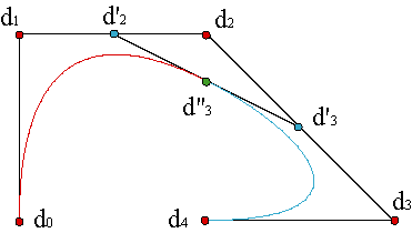
The iterated application of the insertion algorithm of the knots ui,ui+1 until they reach the multiplicity n is an equivalent way of obtaining the control polygon of the curve over the interval [ui,ui+1]. Example.
This seems clear because the list of knots of that interval after the insertion will be:
{ui < n > , ui+1 < n > } and that corresponds to a Bézier curve with vertices:
ci = d[ui < n-i > , ui+1 < i > ].
We may elevate the degree of B-splines in (almost) the same way as we elevate the degree of Bézier curves using:
| |||||||
which associates the blossom of a curve of degree n with the blossom of degree n+1 for the same curve.
Expression (19) was derived for Bézier curves and therefore it makes no reference to any sequence of knots.
A given B-spline is a piecewise degree n curve over a given knot sequence: {u0 < n > , u1 < n > } . Its differentiability is determined by knot multiplicities. If we write it as a piecewise curve of degree n+1, we need to increase the multiplicity of every knot by one, thus keeping the original differentiability properties. Hence the sequence of knots will be {u0 < n+1 > , u1 < n+1 > }.
Consequently, in order to elevate the degree we have to use formula (19), but taking into account that we have to duplicate every inner knot: from un-1 to un+N-1. Example.
In order to elevate the degree of a piecewise polynomial curve we use expression (19), for instance, for finding the B-spline polygon° with the knot sequence,
| |||||
and we finally obtain 2n+2N knots and n+2N vertices.
In chapter two, we proved that the derivatives of a Bézier curve could be expressed by the blossom:
| |||||||||
using vectorial interpolations with vector e, that connects the points 0 and 1 over the real line.
This expression is still acceptable for every piece of a spline curve, because it is based on the blossom. For instance, the first derivative in u ∊ [ui,ui+1],
| |||||||||||
That is, the vertices of the last step of the algorithm determine the tangent directions to the curve at c(u). Example. For higher derivatives,
| |||||||||||
And if we have piecewise polynomial curves of degree n, the curve c(u) is Cn-1 at ui, if this knot is simple.
In case of multiple knots is not much complicated. Example.
This result shows the versatility of piecewise polynomial curves, which allow us to combine pieces with different classes of differentiability by repeating the knots at the unions.
As the iterated application of the de Casteljau algorithm introduces the Bernstein polynomials, the de Boor algorithm introduces polynomial functions in each piece.
Consider piecewise polynomial functions defined over [u0,um], with partition {u0,...,um}, such that inside each interval [ui,ui+1] the functions are polynomials of degree n and at every knot ui they are Cn-ri. This functions form a linear space.
The dimension of the spline function space of degree n and N pieces is dim = n+N = 1+L, that is, it is equal to the number of vertices of the B-spline polygon.
We can encode the de Boor algorithm in some functions {Nn0(u),..., NnL(u)}, basis of that space, such that the polygon of the curve is {d0,..., dL},
| |||||
In order to do that, we have to construct functions instead of parametric curves.
Expressing the linear monomial u with the blossom,
| ||||
elevating the blossom to degree n, we obtain
| |||||||||
Hence, in order to find the B-spline polygon, {ξ0,...,ξn+N-1}, of the linear monomial with a sequence of knots {u0,...,u2n+N-2}, degree n and N pieces, we evaluate the blossom
| |||||||
These terms are called Greville abscissae.
Therefore, if we express a piecewise polynomial function f(u), as a graphic, (u,f(u)), the vertices of its B-spline control polygon will be of the form (ξi,[d']i), where [d']i are the vertices of the parametric "curve'' f(u).
With that information, we construct the B-spline functions, Nni(u), of degree n over a sequence of knots {u0,...,u2n+N-2} in the same way as those of the graphic which has as B-spline polygon {di0,...,din+N-1}, where dij = (ξj,Δij), that is, the ordinate of every vertex is null, but the one corresponding to index i.
Hence, {Δi0,...,Δin+N-1} is the polygon of the nodal function Nni(u).
Therefore,
{ΣdiΔi0,...,ΣdiΔin+N-1} = {d0,...,dn+N-1} is, at
the same time, the polygon of c(u) and ΣdiNni(u),. Consequently we have arrived to
expression (24).
B-spline functions are piecewise polynomials.
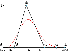
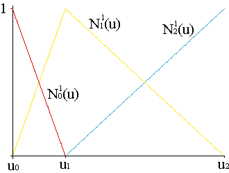
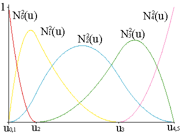
Consider the graphic of the function Nni(u) over a sequence of knots {u0,...,u2n+N-2}.
The support, the closed interval out of which the function Nni(u) is null, is [ui-1,ui+n]. A major property of these functions is that they have minimal support. There are no non-null functions with smaller support than the B-spline functions.
All of these are linearly independent, hence, the B-spline functions form a basis for this space.
And B-spline functions form a partition of unity, as Bernstein polynomials,
| (27) |
Just as the de Casteljau algorithm for Bézier curves is related to the recursion of Bernstein polynomials, the de Boor algorithm yields a recursion for B-splines,
| ||||||||||||||||||||||||||||
for a given sequence of indices {u0,...,u2n+N-2}. Example.
As we said, iterated application of the de Boor algorithm to rational curves introduces an auxiliary coordinate that gives place to the denominator of the parametrization.
In the same way, a piecewise rational curve could be expressed in terms of B-spline functions introducing a denominator.
Hence, a rational degree n curve with N pieces is determined by the vertices of its B-spline polygon , {d0,...,dn+N-1}, the corresponding weights, {w0,...,wn+N-1}, and a sequence of knots, {u0,...,u2n+N-2},
| ||||||
The procedures derived for piecewise polynomial curves as knot insertion, degree elevation... can be automatically translated to rational curves by introducing an auxiliary coordinate and projecting.
Because of local control property, modification of a weight changes only n+1 pieces of the curve. Example. The properties of rational curves hold, and of course, those of piecewise polynomials.