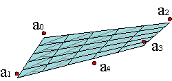
Surface design should be more complicated than curve design. However, we shall make use of many of the tools and algorithms that we have studied up to this moment.
Consider a spatial polynomial curve with control polygon given by {c0,..., cm}, ci ∊ A3. It is represented as:
| ||||
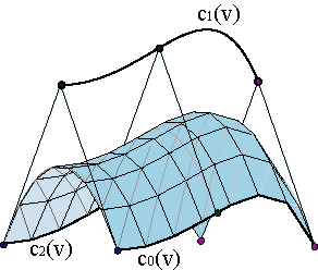
If we allow the control polygon vertices to move along parametrized curves ci(v),
| ||||
the Bézier curves c(u,v0), with polygons {c0(v0),..., cm(v0)}, evolve through the space describing a parametrized surface c(u,v). Example.

We are interested in the evolution of vertices along non-arbitrary curves ci(v) but Bézier curves of degree n with respective control polygons {ci,0,...,ci,n}. Then the parametrization,
| |||||
describes a surface of degree (m,n) defined by a control net of (m+1)(n+1) vertices, {c0,0,...,cm,n}.
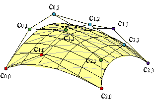
The constant parameter u curves,
| ||||
are Bézier curves of degree n with polygons of vertices cj = (Σici,jBmi(u0)).
While the v constant parameter curves,
| ||||
are Bézier curves of degree m with polygons of vertices ci = (Σjci,jBnj(v0)).
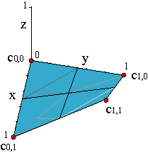
As with non-parametric curves, we can represent graphics of polynomial functions of two variables, f(u,v), because they can be parametrized as c(u,v) = (u,v,f(u,v)).
If we describe f(x,y) as a combination of a control net on the real line, { c'0,0,..., c'm,n}, the graphic of the function will be determined by the control net { c0,0,..., cm,n}, whose vertices are
| (2) |
The tensor product representation can be adapted in order to construct B-spline surfaces. The only thing we have to do is to replace Bernstein polynomials by B-spline functions.
Hence, in order to determine a B-spline surface of degree (m,n) with MxN pieces, we should provide two sequences of knots, {u0,..., u2m+M-2}, {v0,..., u2n+N-2} and a control net formed by the vertices {d0,0,...,dm+M-1,n+N-1}. The parametrization,
| (3) |
is defined over the interval [um-1,um+M-1]x[vn-1,vn+N-1].
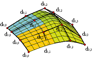
As with B-spline curves, it is usual that the knot sequence begins and ends with m and n knots repeated.
Even introducing weights {wi,j} does not disturb at all on defining rational and piecewise rational surfaces,
| (4) |
that allow us, for example, to describe in an precise way a cylinder, for example.
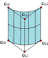
| (5) |
As a generalization of polynomial curves, Bézier surfaces inherit most of their properties.
| (6) |
our basis of functions is a partition of unity as well.
Affine invariance:
| |||||
for each and every affine map f. Besides rational surfaces are projectively invariant.
Convex hull property of the control net: the surface is included in the convex hull of the control net. Example. For piecewise surfaces, every piece is included in the convex hull of their control net.
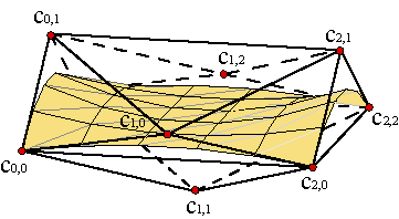
Diminishing variation property: This property is not inherited from the univariate case. Counting intersections with straight lines, as we did for curves, would not make Bézier patches variation diminishing. It is easy to construct a patch that is intersected by a straight line while its control net is not.
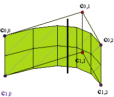
In order to redefine the parametrization over a rectangular set, [a,b]x[c,d], different from [0,1]x[0,1], we just reparametrize:
| ||||||||
Consequently, the new parametrization will be:
| ||||||||
As Bézier curves pass through the first and last vertices, corresponding to t = 0, t = 1, Bézier surfaces pass through the four vertices that lie at the four corners of the control net,
| ||||
Furthermore: the four Bézier curves that formed the corners of the control net lie on the patch. For instance, if u = 0,
| ||||
The corresponding curve c(0,v), has as control polygon {c0,0,..., c0,n}: it is the first row of the control net of the surface. At the same time, the last row, {cm,0,..., cm,n}, is the control polygon of the curve c(1,v). And for v = 0,
| ||||
the control polygon of the curve c(u,0) is the first column of the control net {c0,0,..., cm,0}. Analogously, the control polygon of c(u,1) is the last row: {c0,n,..., cm,n}.
The curves that form the sides of the control net lie on the patch. Example.
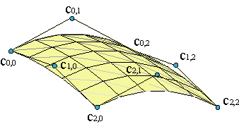
This property works as well with rational and piecewise rational surfaces, if the knots at the beginning and at the end of each piece have multiplicity equal to the degree.
Piecewise surfaces fulfill local control property as well. A generic vertex of the control net affects at most (m+1)·(n+1) pieces of the surface. In the following figure the vertex c3,3 has been displaced. The surface is a surface of degree (2,2) with 5x5 segments. Example.

If a weight is increased, the surface approaches the corresponding vertex of the net. Example.
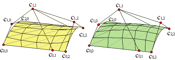
The main inconvenients of the tensor product representation are the limitations on the topology of the surface. If surfaces are open, there is no problem at all, but if they are closed, the only topologies allowed are those of the cylinder and the torus. In order to represent the sphere we have to use degenerate nets whose vertices overlap at the poles.
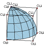
We can easily extend the de Casteljau Algorithm to surfaces: we just apply the algorithm to each column of the control net, as if they were curves of degree m,
| ||||||
until we end with a point at the m-th iteration of each column {cm,0)0,0(u),...,cm,0)0,n(u)}, which can be considered as a curve of degree n.
Applying the algorithm once more,
| ||||||
until we the last iteration, we get the point c(u,v) on the surface,
| |||||
The procedure is symmetric. We can do it with the rows.
The blossom of a Bézier surface is:
| |||||
that is, we evaluate the blossom first at u1,...,um in each column of the control net and we evaluate the resulting polygon of degree n at :v1,...,vn. We can do it first with the rows v1,...,vn and then with the resulting column u1,...,um.
If we want to limit the surface c(u,v) to the interval [a,b]x[c,d], the new control net {c'0,0,..., c'm,n} is ,
| |||||
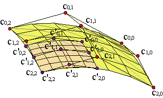
A surface of degree (m,n) and control net, {c0,0,...,cm,n}, can be described as a surface of degree (m+1,n) just applying the degree elevation algorithm to the n+1 columns of the control net independently,
| |||||
| |||||||||
Analogously, if we want to express this surface as of degree (m,n+1), we just apply the degree elevation algorithm to the m+1 rows of the control net independently,
| |||||
| |||||||||
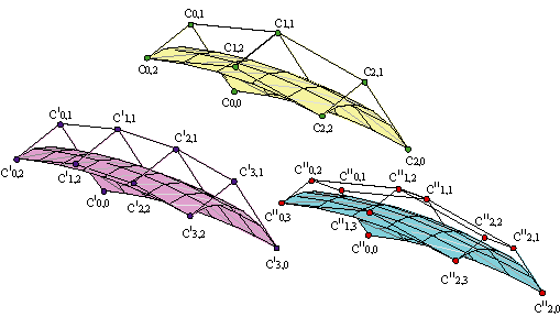
We can extend it to the rest of the formulae: blossom and repeated degree elevation.
For curves, derivatives were carried out by taking differences of control points. We shall consider partial derivatives with respect to the variables u,v in Bmi(u)Bnj(v).
For instance, the partial derivative with respect to u,
| |||||||
where:
| ||||
the first values are the generalization of the standard difference operator with just one index,
| ||||
The partial derivative with respect to v is
| |||||||
| |||||||||
We can evaluate it along isoparametric lines. The ones on the boundary are those of most interest: for u = 0, u = 1, v = 0, v = 1.
Consider the case: u = 0. A partial derivative is the tangent vector of an isoparametric curve.
This derivative is called cross boundary derivative along the edge v = 0. The cross boundary derivative depends on only two rows.
Cross boundary derivatives with respect to u:
| |||||||||
For instance, for u = 1,
| |||||||||
We shall make use of these results for constructing polynomial patches.
Given two Bézier surfaces parametrized by c(u,v) and c'(u,v), respectively, over the intervals [u0,u1]x[v0,v1], [u1,u2]x[v0,v1], with control nets {c0,0,..., cm,n} and { c'0,0,..., c'm,n}, and linked by a common boundary u = u1, the condition of continuity implies that the curves c(u1,v), c'(u1,v) must be the same, i. e., the last row of the first control net and the first row of the second one are the same:
| (22) |
They are differentiable with continuity (C1 ) across their common boundary curve if (see 20-21),
| ||||||||
| (23) |
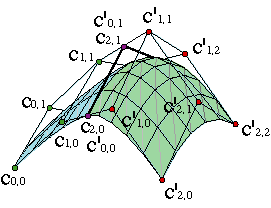
We can interpret it if we think of the columns of the nets {c0,j,..., cm,j}, { c'0,j,..., c'm,j} as control polygons of piecewise curves to which we are imposing the condition of having continuous first derivative.
Consequently, the C1 condition affects the vertices of the last two rows of the first surface and the first two rows of the second surface.
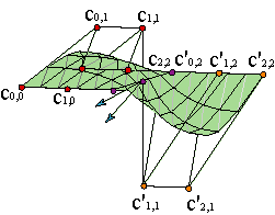
However, if we impose instead of (23) the pair of vectors Δ1,0 cm,j, Δ1,0 c'0,j to be parallel, we get a surface that in general does not even have a tangent plane at the points of the boundary, but at the endpoints (this can be verified calculating the normal vector along the boundary).
The Cr condition for piecewise surfaces is:
| (24) |
From formula 19 for r=s=1, we obtain a mixed partial which is known as the twist. The twist of a surface is its mixed partial derivative ∂2/∂u∂v:
| |||||||
We can re-write the coefficients in order to obtain a easy geometrical interpretation:
| ||||
| ||||
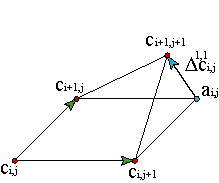
The vector Δ1,1ci,j represents the deviation of the vertex ci+1,j+1 with respect to the parallelogram determined by ci,j, ci+1,j,ci,j+1,ai,j.
At the corners of the boundary of the surface, for instance, at c0,0, the twist is proportional to Δ1,1c0,0 and, as the vectors c0,0c1,0, c0,0c0,1 determine the tangent plane at c0,0, the twist vector is a measure of the deviation of c1,1 from the tangent plane at c0,0.
A bicubic Bézier surface has a control net with 16 vertices, of which 12, the outer ones, are determined by the curves on the boundary. Thus, we only have freedom for choosing the 4 inner vertices which could be determined if we fix the twists of the corners. Hence, choosing the twists is fundamental in order to determine the surface that fills in the space between four curves.

The easiest choice is taking null twists. The surfaces with null twists are called translational surfaces. Example.
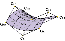
We can use the derivatives of the parametrization for constructing normal vectors to the surface. The normal vector of a surface is a normalized vector that is orthogonal to the surface at a given point. It can be computed from the cross product of any pair of vectors that are tangent to the surface at that point. We may set:
| ||||||||
This expression, normalized, is the normal vector.
It is not valid if partial derivatives are parallel or null.
At the four corners of the patch, the involved partial derivatives are simply differences of boundary points. For example, at c0,0 = c(0,0),
| (26) |
The normal at one of the corners is undefined if c0,0, c0,1, c1,0 are linearly dependent (collinear).
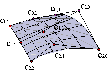
Assume that we are given an array of (m+1)·(n+1) data points in space: {a0,0,..., am,n}, and we want a surface c(u,v) to interpolate them,
| (27) |
We try a tensor product patch of degree (m,n). We can describe it as BUCBVt = A,
| ||||||||||||||||||||||||
| ||||||||||||||||||||||||
| ||||||||||||||||||||||||
| ||||||||||||||||||||||||
where the matrices A,C define three linear systems.
The coordinates of the vertices of the control net can be obtained inverting the matrices
C = BU-1A(BVt)-1.
However, it is easier to define auxiliary matrices (interpolating curves approach) C': = BUC, which will be the unknowns of the system C'BVt = A.
Thus, the tensor product formalism allows a significant "compactification" of the interpolation process. Without it, we would have to solve a linear system of order (m+1)·(n+1) instead of solving two systems of respectively (m+1) and (n+1) equations. Example.
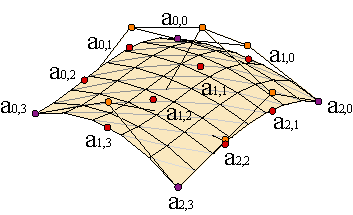
Another option is using bicubic B-spline patches. The philosophy is the same but introducing B-spline functions instead of Bernstein polynomials.
Assume that our given data must satisfy ai,j = c(ui,vj), for i = 0,...,M, j = 0,...,N. We can fix ui and interpolate a cubic spline through the points of the corresponding row {ai,0,...,ai,N}.
We shall obtain M+1 B-spline polygons, one for each row, that form a matrix of points { d'0,0,..., d'M,N+2}. Interpolating with cubic splines each column { d'0,j,..., d'M,j} we obtain a family of N+3 B-spline polygons, {d0,0,..., dM+2,N+2}, that form the B-spline net of the interpolant surface.
The knot sequences are {u0,..., uM}, {v0,..., vN}, with the initial and final knots repeated three times.
Obviously we have to impose further conditions in order to obtain a unique solution.
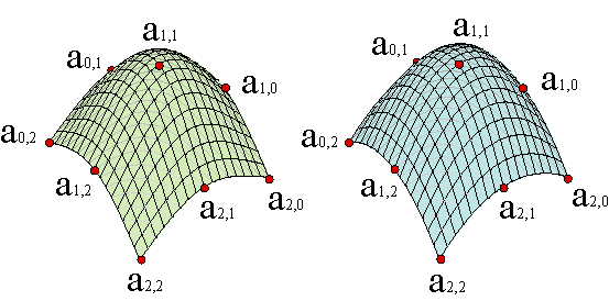
In general, we must expect a problem with unstructured data: we must assign to the data ai some parameters (ui,vi) that do not conform a rectangular net.
Consider the approximation problem for obtaining a surface of degree (m,n) that approximates a given set of data, {a0,...,aM}, such that ai = c(ui,vi). The linear system of the problem,
| (28) |
has (m+1)·(n+1) unknowns for M+1 equations. Hence, the system is overdetermined.
We try a least squares approximation.
If we write our system as BC = A, we can transform it into (m+1)·(n+1) equations with the same number of unknowns,
| (29) |
Although it is in principle solvable, for a large number of data it is bad conditioned.
