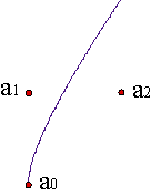
In curve and surface design it is convenient to use simple representations of curves and surfaces. We could represent polynomial curves of degree n by:
| ||||
where each coefficient ai is a point of the plane or the space, depending on whether the curve is planar or spatial.
This representation is not much practical, because it does not give us any clue about the behaviour of the curve.

On the other hand, if we rotate, translate, etc... the curve, the behaviour of its coefficients is impossible to foretell. Example.
Besides, this representation is not stable under little changes (in order to
make a later computation). Example.
Consequently, it seems convenient to adopt other representations of polynomial curves.
We will express polynomials of degree n in terms of Bernstein polynomials,
| |||||||||||||
where Bni(t) is the i-th Bernstein polynomial of degree n. They all have the same degree.
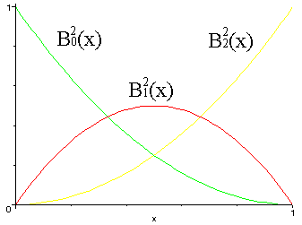
We can represent all polynomial curves of degree n as combinations of these polynomials
| |||||||
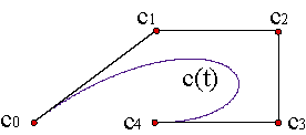
where the coefficients ci are points of the plane or the affine space depending on whether the curve is planar or spatial. These coefficients are called vertices of the control polygon , {c0,...,cn}, of the Bézier curve c(t). Therefore, a curve of degree n has a control polygon of n+1 vertices.
Invariance under affine parameter transformations: Although we have defined the curve in the interval [0,1], it is possible to reparametrize the interval to an interval [a,b],
| ||||||
such that u = a corresponds to t = 0 and u = b, to t = 1. The new reparametrization will be, then,
| ||||||
The curve passes through the vertices c0, cn,
| ||||
In fact, they are the only vertices the curve is passing through. Example.
Local Control: The control polygon serves to control the form of the curve but in a local way: if we pull/push a vertex, all the curve is moving along with it, but mainly the part of the curve closest to such vertex. Example.
Convex hull property: the whole curve is included in the convex hull of the control polygon. Example.
Affine transformations:
| ||||||
the image of the curve by an affine map is quite simple: the image curve has as control polygon the image of the primitive control polygon, {f(c0),..., f(cn)}. Example.
Symmetry: Bézier curves are symmetric. If we reverse the control polygon, {cn,...,c0}, the graph of the curve is the same as the one with control polygon {c0,...,cn}. Example.
The usual way of tracing out Bézier curves is based on the de Casteljau algorithm.
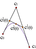
The de Casteljau algorithm is an iterated application of linear interpolation to the control polygon of a Bézier curve,
| |||||
The number of vertices decreases a unity every step,
| |||||
until it ends in a single point at the n-th iteration. Example
| |||||
The advantages of the de Casteljau algorithm are simplicity and the fact that it involves only sums, since every term is positive. Example of a parabola. Example of a cubic.
A very useful construction based on the algorithm of de Casteljau is the blossom.
This is the idea: instead of interpolating always at the same value of t in the n steps of the algorithm, we interpolate with the value t1 in the first step, with t2 in the second, an so... an with the value tn in the last one. We obtain a point c[t1,...,tn]. This point does not correspond to any point of the curve, but in the trivial case when every ti is the same.
Let us see it in a simple example: n = 2, control polygon {c0,c1,c2}:
| |||||||||||||
The blossom is symmetric: c[t1,t2] = c[t2,t1]. This result can be generalized to curves of degree n. Example
The blossom also allows us to rebuild the control polygon of a Bézier curve.
| |||||||
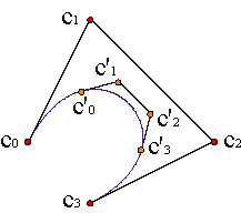
The blossom helps us as well if we want to constrain the interval of definition of a Bézier curve, c(t), defined in the interval [0,1]. If we know the control polygon {c0,...,cn} of the primitive curve, but we do not know that of the curve restricted to the interval [a,b], the vertices of the control polygon of the restricted curve will be
| ||||||||||
In some cases we will be interested in changing the degree of the curve in order to have more freedom in case we would like to modify its form. The curve of degree n and control polygon {c0,..., cn} and the curve of degree n+1 and control polygon {c10,...,c1n+1} whose expression is
| |||||||||
are the same curve. Example
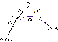
The iteration of the degree elevation process makes the control polygon converge to the curve. Example
Another property is the so called variation diminishing property. A straight line r cuts a Bézier curve, c(t), in at most the same number of points that it cuts the control polygon, {c0,...,cn}. Example
The inverse problem, degree reduction, has not, in general, a solution, because a real curve of degree n+1 cannot be expressed as a curve of degree n, but we can analyse the better aproximation to the problem via least squares approximation.
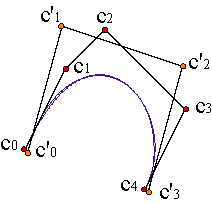
The derivative of a parametrization of a Bézier curve is
| |||||||||
defining the forward difference operator Δ as Δci = ci+1-ci, where ci+1 and ci are vectors.
Hence, the derivative of a parametrization of a Bézier curve of degree n is another parametrization of Bézier of degree n-1, for a given vector curve of given control polygon {Δc0,...,Δcn-1}.
As the curve passes through the first and last vertices, we find that
| |||||||||
The initial and final pair of vertices provide the tangents at the endpoints of the curve. Example
This expression can be generalized to higher derivatives by iteration:
| ||||||||||||||
where the iterated forward difference operator Δs is defined by: Δsci = Δs-1ci+1-Δs-1ci.
Assume that we want to link two Bézier curves of degree n, defined by the adjacent intervals [u0,u1], [u1,u2], with control polygons {c0,..., cn}, {c'0,..., c'n} respectively. If we want continuity, then c(u1) = c'(u1), i. e., cn = c'0.
Besides, if we want the piecewise curve defined over the interval [u0,u2] to be class C1, that is, with a continuous tangent, it should fulfill:
| ||||||||
where: Δ0 = u1-u0, Δ1 = u2-u1.
The condition on the derivatives leads us to a condition on the differences of the vertices.
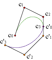
Iterating, the condition for being Cr is:
| |||||||||
Bézier curves can solve the problem of point data interpolation. Let {a0,...,an} n+1 points and we want to obtain the curve c(t) defined over the interval [0,1] that verifies:
| ||||
for given t0,..., tn parameter values.
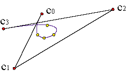
In order to solve the problem, we should find the control polygon of the curve of degree n that verifies the expression:
| ||||||
Hence, we have to solve a linear system of n+1 equations
| ||||||||||||||||||||||||||||||||||||||||
That we can represent as BC = A, where B stands for the matrix of the values of Bernstein polynomials at t0,... ,tn,
and C,A are the matrices whose rows are, respectively, the vertices of the control polygon of the given curve and the solution curve.
The formal solution would be C = B-1A, although the most efficient way of obtaining it should be by some numerical algorithm. Ejemplo.
Finally, a small application for point data interpolation where we can check the issues we have just seen up to this moment.
In many problems we are given more data points that can be interpolated by a polynomial curve. For instance, we have m+1 points and we want to get a n degree curve that fits, as much as possible, the given data points. In such cases an approximating curve will be needed. Such a curve does not pass through the data points exactly; rather, it passes near them, still capturing the shape inherent to the given data points. The best known technique for finding such curve is known as least squares approximation.
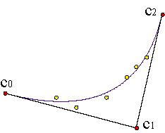
Instead of solving the linear system BC = A, with m+1 equations and n+1 unknowns, we must solve the linear system: BtBC = BtA, that is a system with n+1 equations and n+1 unknowns. Example.