CHAPTER 3: RATIONAL CURVES

1  Introduction

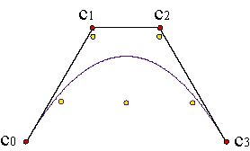
Although the polynomial curves are the easiest tool for curve design, they lack flexibility (for instance, they have as many roots as its degree). Let us see, as an example, how a cubic approximates five points over a sinusoidal curve:

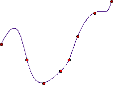
The lack of flexibility of the polynomials can cause, as well, the existence of parts of the curve with a high degree of curvature or undesirable and rough oscillations:

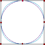
On the other hand, the amount of curves that can be described in an precise way by polynomial parametrizations is quite limited. The result of  approximating a circle by pieces of parabolas is, at least, unsatisfactory:

An alternative possibility, that we will consider in the next chapter, is working with piecewise polynomial curves and functions. Another possibility is using rational curves.

2  Rational Curves 

We shall define the rational parametrizations of degree n as those whose components are polynomial curves of degree n.

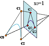
Let (c₀(t),c₁(t),c₂(t)), t∊[0,1] be a polynomial curve in R³ such that does not pass through the origin. We know that its projection onto the affine plane is a parametrization (c₁(t)/c₀(t),c₂(t)/c₀(t)).

We shall split the coordinates of the vertices in two parts: c_i = (w_i,w_ic_i), where  w_i is the first component of the i-th vertex, and w_ic_i are the two remaining components (three, if we are working with a spatial curve). c_i is just the projection of c_i over the affine plane.

In this case, we are describing the rational curves via a control polygon {c₀,...,c_n} and some parameters, {w_i,...,w_n}, that we shall call weights.

If all the wieghts have the same value, w = w_i, i = 0,...,n, then we recover the polynomial curve,

of control polygon {c₀,...,c_n}.

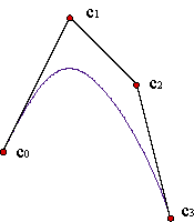
If we want to continue working with positive expressions, we need to use positive values for the weights as well. In design it is usual working with weight values around one. Here is an example of a curve with some negative weights.

The interpretation of the weights is this: The larger the weight w_k is (leaving unchanged the rest of weights), the closer the curve approaches the corresponding vertex c_k . Example 

This fact can be used to increase the "tension" of the curve. Example

If we multiply all the weights by the same factor, the curve remains the same. Example

This well known fact can be used for normalizing the weights by taking the first weight equal to one.

What if one of the vertices c_i is a point at infinity?

In this case, there is no sense in talking about the weight w_i, because the first component of the vertex is equal to zero, c_i = (0,c_i). Its image is an affine vector, not a point, and therefore, we shall call it control vector. Hence, making this distinction, the expression of a rational curve is:

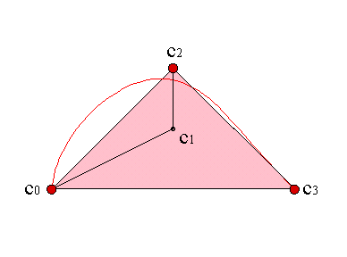
The presence of control vectors is quite disturbing because, the expression (2) is no longer a barycentric combination of points, and, consequently, the property of convex hull will be no longer true. Example

2.1  Properties of Rational Curves

Many of the properties of Bézier curves can be straightaway translated to rational ones, because we are still using barycentric combinations of the control polygon vertices.

The following properties, derived from this fact, remain the same: the convex hull property, the variation diminishing property and the invariance under affine maps. Example

Other properties, as passing through the first and the last vertices c₀, c_n or being symmetric, remain the same as well.

The rational curves are invariant under projective maps. Let f be a projective map of the plane and {c₀,...,c_n}, {w₀,...,w_n} the control polygon and the list of weights of a rational parametrization. Consequently: 

where the vertices and weights c_i = (w_i,w_ic_i) of the transformed curve are related to those of the original curve c_i = (w_i,w_ic_i) by the relation: c'_i = f(c_i) = (w'_i,w'_ic'_i). 

This maps are particular useful because they include the change of perspective. Example

A projective map of the real line transforms a rational parametrization of degree n c(t) into another of the same degree c'(u) = c(t(u)),

We shall reparametrize making keeping the final interval equal to [0,1]. This can be done with transformations of this form:

and this is impossible with affine maps.

These transformations cause the changes of the weights: {w'₀,...,w'_n}, w'_i = b^n-iw_i. But the control polygon remains the same, {c₀,...,c_n}.

There are infinite lists of weights that give us the same rational curve. The graphic of the curve is the same, but the velocity of the parametrization is different.

If b < 1, we travel along the curve faster at the beginning than at the end. When we reach u = 1/2, we are beyond t = 1/2 in the original parametrization. And the contrary happens when b > 1. Example In the following graphic we can see t(u) for b=1/2, green and  b=2, red.

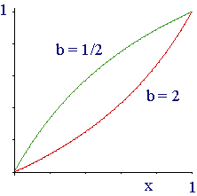
We can freely choose the value of b in order to fix a value for a particular weight. If we choose b = (w_n/w₀)^1/n, then w'₀ = w_n = w'_n.

Usually the initial and final weights are chosen in a way that w₀ = 1 = w_n.

3  Conics

Rational parametrizations describe arcs of any sort of conic sections. 

Assume w₀ = 1 = w₂, w₁ = w (a normalized parametrization), on a rational curve of degree two,

Considering  only positive values of the weights, for 0 < w < 1 we shall get an arch of ellipse. For w = 1, we have an arc of parabola, and for w > 1, we have a hyperbola. Example

With a simple geometrical construction, we can find the vertices of the control polygon of an arc of circumference.

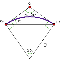
In the figure, if we put the centre in (0,0) and the endpoints c₀, c₂ in (-Rsinα,Rcosα), (Rsinα,Rcosα), respectively, the vertex c₁ will be (0,R/cosα).

The value of the weight is w = cosα. For example, in order to trace a quarter of a circumference, the weight takes the value 2^1/2/2 and for and arch of 2π/3, takes 1/2.

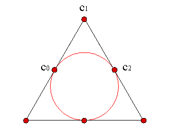
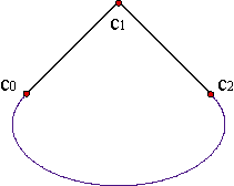
For half a circumference, we can trace it if we use control vectors, Example

4  Degree Elevation

If we multiply both numerator and denominator by the same function f(t), the parametrization is invariant, but both expressions change notably. As our purpose is increasing the degree in one, we choose a function of degree one,

Using this expression, we have countless ways of increasing in one degree the parametrization's degree. It depends on the value of the parameters α,β. It is reasonable to choose them both positive in order to avoid negative terms. Example

If we take α = 1 = β, we get the degree elevation formula derived in the previous chapter (Chapter 2).

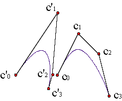
Degree elevation (5) and (4) are not commutative. This means that if we first increase the degree of the curve and then reparametrize, we shall not get the same result as if we first reparametrize and then increase the degree of the curve, as it can be seen in the following figure: 

5  The de Casteljau Algorithm

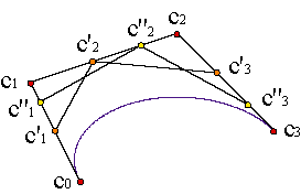
The de Casteljau Algorithm can be generalized to rational curves:

where, obviously, w⁰⁾_i = w_i, c⁰⁾_i = c_i.

6  Derivatives

For a given control polygon {c₀,... ,c_n}, and a list of weights, {w₀,... ,w_n},

the expression of the derivatives of a product give us the derivative of the rational parametrization,

These expressions are very intricate, because they involve lower derivatives in both numerator and denominator.

Due to the formulae for the derivatives of the polynomial parametrizations,

regarding the first derivative there is only one new thing, the weights of the first and the last point. Example

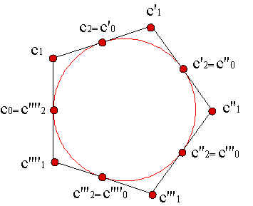
Let {c₀,... ,c_n}, {c'₀,... ,c'_n} and {w₀,... ,w_n}, {w'₀,...,w'_n} be the control polygons and list of weights of two rational curves defined over the intervals [u₀,u₁] and [u₁,u₂] respectively. The condition for forming a continuous curve is:

This is the same condition studied for Bézier curves.

As c_n, c'₀ are the same point, it seems reasonable to impose w_n = w'₀.

Besides, if we want the parametrization to be C¹ class, 

From the second derivative on, things get more complicated. If we want the rational parametrization to be C^r class, we can impose a sufficient condition, but not necessary, in order to achieve our goal:

7  Interpolation and approximation

Rational curves add many degrees of freedom to those of Bézier curves, and we shall use them in order to solve more complex problems of interpolation and approximation.

We could see the rational problem as a polynomial problem in R³ where the given data are the values c(t_i) = a_i, i = 0,...,m, for a_i = (v_i,v_ia_i). As the given data of the problem are: c(t_i) = a_i, consequently, the weights of the given points v_i, i = 0,...,m remain as free parameters.

There are no general algorithms to determine those weights. Thus we are to consider them as degrees of freedom that will allow us to improve the resulting curve. Example